Ising Model
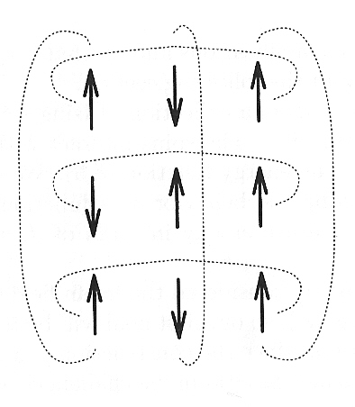
The two-dimensional Ising model is defined by \begin{equation} H = -\frac{1}{2}\sum_{ij} J_{ij} S_i S_j = -\sum_{\langle i j \rangle} J_{ij} S_i S_j. \end{equation} We take $J_{ij}=J=1$ for nearest neighbors and $J_{ij}=0$ otherwise. Each spin has the value $S_i=\pm1$, and we use units with $k_B=1$.
On an $L\times L$ lattice, choose a site uniformly at random and propose flipping its spin. Thus, $\omega_{XX'}=1/L^2$ when $X$ and $X'$ differ by one spin flip, and $\omega_{XX'}=0$ otherwise.
The energy difference $\Delta E=E(X')-E(X)$ is inexpensive to calculate because only the four bonds connected to the selected spin change. If $\Delta E<0$, the trial state is accepted; if $\Delta E>0$, it is accepted with probability $\exp(-\beta\Delta E)$.
Keep in mind:
- The total energy and magnetization need to be computed from scratch only for the initial configuration. After every accepted spin flip, both can be updated using their changes.
- At fixed temperature, $\exp(-\beta\Delta E)$ takes only five possible values. It is therefore useful to precompute these values.
- One Monte Carlo sweep means $L^2$ attempted spin flips. It is more informative to quote equilibration and measurement intervals in sweeps rather than individual attempted flips.
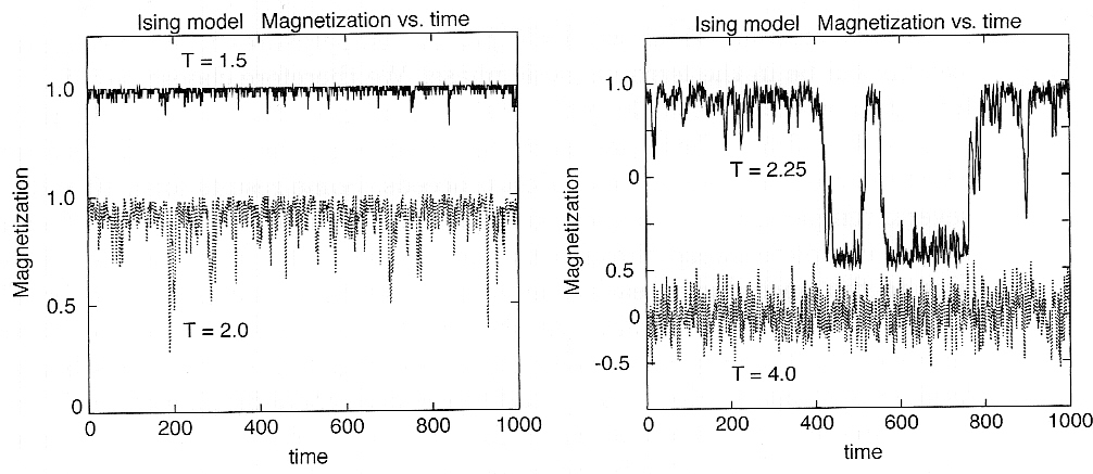
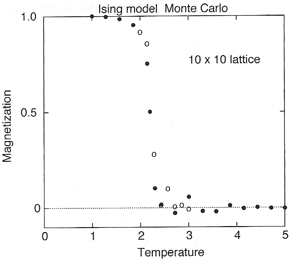
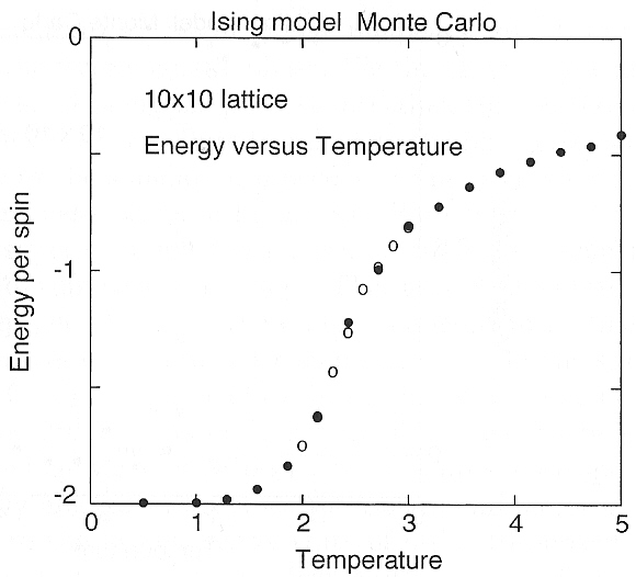
- The exact transition temperature is $T_c/J=2/\ln(1+\sqrt{2})\approx2.26919$, or $\beta_cJ\approx0.440687$. Local Metropolis updates become strongly correlated near $T_c$ (critical slowing down).
- A cooling scan should agree with a heating scan within statistical errors. A visible difference is a warning that the simulation has not equilibrated.
Algorithm
Choose temperature $T$ and precompute the exponents $[\exp(-8J/T),\exp(-4J/T),1,\exp(4J/T),\exp(8J/T)]$.
Generate a random configuration $X_0$, corresponding to infinite temperature.
Compute the total energy and magnetization of $X_0$.
Repeat the following update many times:
- Select a spin uniformly at random and compute its Weiss field, $W_i=\sum_{j\text{ neighbor of }i}J_{ij}S_j$.
- Flipping the spin changes the energy by $\Delta E=2S_iW_i$. Use the precomputed exponents to evaluate $P=\min(1,\exp(-\Delta E/T))$.
- Accept the trial step with probability $P$. If accepted, set $S_i\leftarrow-S_i$, $E\leftarrow E+\Delta E$, and $M\leftarrow M-2S_i$, where $S_i$ on the right is the old spin.
- After equilibration, measure $E$, $E^2$, $M$, $M^2$, and $|M|$ at regular intervals. Measure after attempted updates, not only after accepted updates: rejected steps also belong to the Markov chain.
For $N_s=L^2$ spins, we report quantities per spin:
- $e=\langle E\rangle/N_s$ and $m=\langle|M|\rangle/N_s$. For a finite system at zero field, spin-inversion symmetry gives $\langle M\rangle=0$, so $\langle|M|\rangle$ is more useful for displaying magnetic order.
- $c_V=(\langle E^2\rangle-\langle E\rangle^2)/(N_sT^2)$.
- $\chi=(\langle M^2\rangle-\langle M\rangle^2)/(N_sT)$.
Successive measurements are correlated. We group them into blocks longer than the autocorrelation time and use a delete-one-block jackknife to estimate statistical errors. The estimated errors should be checked for stability as the block length is increased.
The fluctuation formula for the total heat capacity follows from \begin{equation} C_V=\frac{\partial\langle E\rangle}{\partial T}=\frac{\langle E^2\rangle-\langle E\rangle^2}{T^2}. \end{equation} Likewise, if the Hamiltonian in a magnetic field is $H-hM$, the zero-field susceptibility is \begin{equation} \chi=\left.\frac{\partial\langle M\rangle}{\partial h}\right|_{h=0}=\frac{\langle M^2\rangle-\langle M\rangle^2}{T}. \end{equation} The code divides these extensive quantities by $N_s=L^2$ to report the heat capacity and susceptibility per spin.
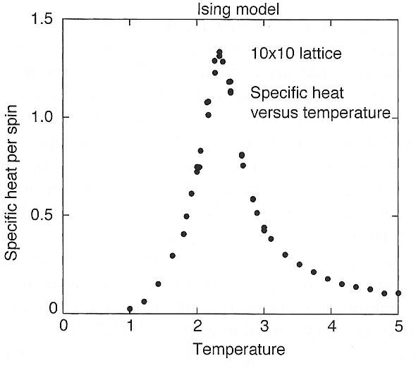
Simulation of the Ising model
import matplotlib.pyplot as plt
import numpy as np
from numba import jit

rng = np.random.default_rng(509)
N = 20  # lattice size: N x N

@jit(nopython=True)
def CEnergy(latt):
    """Return the total energy of a square Ising lattice with J=1."""
    energy = 0
    N = len(latt)
    for i in range(N):
        for j in range(N):
            spin = latt[i,j]
            # right, above, left, and below, with periodic boundaries
            field = (latt[(i+1)%N,j] + latt[i,(j+1)%N] + latt[(i-1)%N,j] + latt[i,(j-1)%N])
            energy -= field*spin
    return energy/2.0  # every bond was counted twice

def RandomL(N):
    """Return a random lattice, corresponding to infinite temperature."""
    return rng.choice((-1,1), size=(N,N))

def Exponents(T):
    PW = np.zeros(9, dtype=float)
    # Precomputed exponents: PW[4+x] = exp(-2*x/T), where x=S_i*W_i.
    PW[4+4] = np.exp(-4.*2/T)
    PW[4+2] = np.exp(-2.*2/T)
    PW[4+0] = 1.0
    PW[4-2] = np.exp( 2.*2/T)
    PW[4-4] = np.exp( 4.*2/T)
    return PW
latt = RandomL(N)
print(latt)
print('Energy=', CEnergy(latt))
T=2.269
PW = Exponents(T)

print('Exponents=', PW)
[[ 1 -1  1  1  1  1  1  1 -1  1  1 -1 -1 -1 -1 -1 -1 -1  1  1]
 [-1 -1 -1 -1  1  1 -1  1 -1  1 -1  1  1 -1  1  1  1  1 -1 -1]
 [ 1  1  1  1  1 -1  1 -1 -1 -1  1  1  1 -1 -1  1  1  1 -1  1]
 [ 1 -1  1  1 -1 -1 -1 -1 -1 -1  1 -1  1 -1  1 -1 -1  1  1 -1]
 [-1 -1  1  1  1  1 -1 -1  1  1 -1 -1 -1 -1 -1  1  1  1  1 -1]
 [ 1  1 -1 -1 -1 -1  1 -1 -1  1 -1 -1 -1 -1 -1  1 -1 -1 -1  1]
 [ 1  1 -1  1 -1 -1  1 -1  1  1  1  1 -1  1 -1  1  1  1 -1 -1]
 [-1  1  1 -1  1 -1  1 -1  1 -1  1  1 -1  1 -1  1  1  1 -1 -1]
 [-1  1  1 -1  1 -1  1  1 -1  1 -1 -1 -1 -1 -1  1  1 -1 -1 -1]
 [-1  1  1 -1 -1  1  1 -1  1 -1 -1 -1 -1  1  1  1  1  1 -1  1]
 [ 1 -1  1  1 -1  1 -1 -1  1  1 -1 -1  1 -1 -1  1 -1  1 -1  1]
 [-1  1  1 -1 -1  1 -1  1 -1  1 -1 -1  1  1  1  1  1 -1  1  1]
 [ 1  1 -1 -1  1 -1  1 -1 -1 -1 -1 -1  1 -1 -1 -1  1  1 -1 -1]
 [-1 -1 -1  1  1  1 -1  1  1  1  1 -1 -1 -1  1  1 -1 -1 -1  1]
 [ 1 -1 -1  1  1 -1  1  1  1  1 -1  1  1  1 -1 -1 -1 -1  1  1]
 [-1  1  1 -1  1 -1  1  1  1 -1 -1  1 -1 -1 -1 -1 -1  1 -1 -1]
 [-1 -1  1  1  1  1 -1  1  1 -1 -1  1 -1 -1  1  1  1 -1  1 -1]
 [-1  1 -1  1  1  1  1  1 -1  1 -1  1  1 -1  1 -1  1 -1  1  1]
 [ 1  1  1  1 -1  1  1 -1 -1 -1 -1 -1 -1  1 -1 -1  1 -1 -1  1]
 [ 1 -1  1 -1 -1  1 -1  1  1  1  1 -1 -1 -1 -1 -1  1  1  1  1]]
Energy= -16.0
Exponents= [3.39803455e+01 0.00000000e+00 5.82926629e+00 0.00000000e+00
 1.00000000e+00 0.00000000e+00 1.71548176e-01 0.00000000e+00
 2.94287767e-02]
Block jackknife error estimation
Monte Carlo measurements generated by a Markov chain are correlated. We therefore divide the measurements into blocks that are long compared with the autocorrelation time. The blocks can then be treated as approximately independent.
The jackknife constructs several estimates of an observable by removing one complete block at a time. If removing one block changes the result significantly, the statistical uncertainty is large. If all the block-deleted results are similar, the uncertainty is small.
Measurements and blocks
Suppose that we retain $N_{\mathrm{meas}}$ Monte Carlo measurements. For every measurement $i$, we store the five quantities
$$ \mathbf q_i = \left( E_i,\, E_i^2,\, |M_i|,\, M_i,\, M_i^2 \right). $$
We divide the measurements into $B$ blocks, with $L$ measurements in each block:
$$ N_{\mathrm{meas}}=BL, $$
where
$$ B=\texttt{n\_blocks}, \qquad L=\texttt{block\_size}. $$
In the present simulation,
$$ N_{\mathrm{meas}}=6000, \qquad L=300, \qquad B=20. $$
Thus, every block contains 300 measured sweeps.
The full-data average of the five measured quantities is
$$ \overline{\mathbf q} = \frac{1}{N_{\mathrm{meas}}} \sum_{i=0}^{N_{\mathrm{meas}}-1}\mathbf q_i. $$
Explicitly,
$$ \overline{\mathbf q} = \left( \langle E\rangle,\, \langle E^2\rangle,\, \langle |M|\rangle,\, \langle M\rangle,\, \langle M^2\rangle \right). $$
Sum of the measurements in each block
Let block $b$ contain the measurements
$$ i=bL,\ldots,(b+1)L-1, \qquad b=0,\ldots,B-1. $$
Define the sum of the measurements in block $b$ as
$$ \boxed{ \mathbf S_b = \sum_{i=bL}^{(b+1)L-1}\mathbf q_i }. $$
Explicitly,
$$ \mathbf S_b = \left( \sum_{i\in b}E_i,\, \sum_{i\in b}E_i^2,\, \sum_{i\in b}|M_i|,\, \sum_{i\in b}M_i,\, \sum_{i\in b}M_i^2 \right). $$
This is implemented by
block_sums = np.sum(
    data.reshape(n_blocks, block_size, 5),
    axis=1,
)
The total sum over all measurements is
$$ \boxed{ \mathbf S = \sum_{i=0}^{N_{\mathrm{meas}}-1}\mathbf q_i = \sum_{b=0}^{B-1}\mathbf S_b }. $$
In the code, this is
np.sum(data, axis=0)
Leave one block out
For every block $b$, we remove that entire block and recalculate the averages using all remaining measurements.
The sum after removing block $b$ is
$$ \mathbf S^{(-b)} = \mathbf S-\mathbf S_b. $$
The superscript $(-b)$ means “with block (b) removed.”
Because one block contains (L) measurements, the number of measurements that remain is
$$ N_{\mathrm{meas}}-L. $$
The average calculated without block $b$ is therefore
$$\overline{\mathbf q}^{(-b)}= \frac{\mathbf S-\mathbf S_b}{N_{\mathrm{meas}}-L}. $$
This is implemented by
leave_one_out = (
    np.sum(data, axis=0) - block_sums
)/(n_used - block_size)
The row leave_one_out[b] contains
$$ \overline{\mathbf q}^{(-b)} = \left( \langle E\rangle_{(-b)}, \langle E^2\rangle_{(-b)}, \langle |M|\rangle_{(-b)}, \langle M\rangle_{(-b)}, \langle M^2\rangle_{(-b)} \right). $$
Because there are $B$ possible blocks to remove, we obtain $B$ different block-deleted averages:
$$ \overline{\mathbf q}^{(-0)}, \overline{\mathbf q}^{(-1)}, \ldots, \overline{\mathbf q}^{(-(B-1))}. $$
For the current simulation,
$$ N_{\mathrm{meas}}=6000, \qquad L=300, \qquad B=20. $$
Consequently, every leave-one-block-out average contains
$$ 6000-300=5700 $$
measurements.
Recalculate the physical observables
Let $N_s$ denote the number of spins:
$$ N_s=N^2. $$
For every omitted block $b$, we recalculate all four physical observables from the remaining measurements.
The absolute magnetization per spin is
$$ m^{(-b)} = \frac{ \langle |M|\rangle_{(-b)} }{ N_s }. $$
The energy per spin is
$$ e^{(-b)} = \frac{ \langle E\rangle_{(-b)} }{ N_s }. $$
The heat capacity per spin is
$$ c_V^{(-b)} = \frac{ \langle E^2\rangle_{(-b)} - \langle E\rangle_{(-b)}^2 }{ T^2N_s }. $$
The susceptibility per spin is
$$ \chi^{(-b)} = \frac{ \langle M^2\rangle_{(-b)} - \langle M\rangle_{(-b)}^2 }{ TN_s }. $$
We collect the four observables into the vector
$$ \boxed{ \boldsymbol{\theta}^{(-b)} = \left( m^{(-b)}, e^{(-b)}, c_V^{(-b)}, \chi^{(-b)} \right) }. $$
This is implemented by
jackknife_values = np.array([
    ObservablesFromMoments(m, T, n_spins)
    for m in leave_one_out
])
Thus, jackknife_values[b] contains the four observables calculated after removing block $b$.
The shape of jackknife_values is
(n_blocks, 4)
or, mathematically,
$$ B\times4. $$
Jackknife mean
For one observable $\theta$, let $\theta^{(-b)}$ be its value after removing block $b$.
The mean of all the block-deleted estimates is
$$ \boxed{ \overline{\theta}_{\mathrm{JK}} = \frac{1}{B} \sum_{b=0}^{B-1}\theta^{(-b)} }. $$
For all four observables simultaneously, this is implemented by
jackknife_mean = np.mean(jackknife_values, axis=0)
The result is the vector
$$ \overline{\boldsymbol{\theta}}_{\mathrm{JK}} = \left( \overline m_{\mathrm{JK}}, \overline e_{\mathrm{JK}}, \overline{c_V}_{\mathrm{JK}}, \overline\chi_{\mathrm{JK}} \right). $$
The notebook uses the estimate calculated from all measurements as the reported central value. The block-deleted estimates are used to calculate its statistical uncertainty.
Jackknife variance and standard error
The jackknife estimate of the variance of an observable $\theta$ is
$$ \boxed{ \sigma_\theta^2 = \frac{B-1}{B} \sum_{b=0}^{B-1} \left( \theta^{(-b)} - \overline{\theta}_{\mathrm{JK}} \right)^2 }. $$
The jackknife standard error is the square root of this variance:
$$ \boxed{ \sigma_\theta = \sqrt{ \frac{B-1}{B} \sum_{b=0}^{B-1} \left( \theta^{(-b)} - \overline{\theta}_{\mathrm{JK}} \right)^2 } }. $$
This is implemented for all four observables at once by
errors = np.sqrt(
    (n_blocks-1)/n_blocks
    *np.sum(
        (jackknife_values-jackknife_mean)**2,
        axis=0,
    )
)
The returned error array is
$$ \left( \sigma_m, \sigma_e, \sigma_{c_V}, \sigma_\chi \right). $$
Origin of the factor ((B-1)/B)
To understand the prefactor, first consider a simple average of $B$ independent block values:
$$ \overline{x} = \frac{1}{B} \sum_{b=1}^{B}x_b. $$
The sample variance of the individual block values is
$$ s_x^2 = \frac{1}{B-1} \sum_{b=1}^{B} (x_b-\overline{x})^2. $$
The estimated variance of their average is therefore
$$ \sigma_{\overline{x}}^2 = \frac{s_x^2}{B} = \frac{1}{B(B-1)} \sum_{b=1}^{B} (x_b-\overline{x})^2. $$
If block $b$ is removed, the average of the remaining $B-1$ blocks is
$$ \overline{x}^{(-b)} = \frac{1}{B-1} \sum_{\substack{j=1\\j\ne b}}^{B}x_j. $$
Because
$$ \sum_{\substack{j=1\\j\ne b}}^{B}x_j = B\overline{x}-x_b, $$
the leave-one-out average can be written as
$$ \overline{x}^{(-b)} = \frac{ B\overline{x}-x_b }{ B-1 }. $$
For a simple average, the mean of all leave-one-out estimates is equal to the full average:
$$ \overline{x}_{\mathrm{JK}} = \frac{1}{B} \sum_{b=1}^{B}\overline{x}^{(-b)} = \overline{x}. $$
The deviation of one leave-one-out estimate from the jackknife mean is
$$ \begin{aligned} \overline{x}^{(-b)}-\overline{x}_{\mathrm{JK}} &= \frac{B\overline{x}-x_b}{B-1} -\overline{x}\\ &= \frac{\overline{x}-x_b}{B-1}\\ &= -\frac{x_b-\overline{x}}{B-1}. \end{aligned} $$
Squaring this expression gives
$$ \left( \overline{x}^{(-b)}-\overline{x}_{\mathrm{JK}} \right)^2 = \frac{ (x_b-\overline{x})^2 }{ (B-1)^2 }. $$
After summing over all omitted blocks,
$$ \sum_{b=1}^{B} \left( \overline{x}^{(-b)}-\overline{x}_{\mathrm{JK}} \right)^2 = \frac{1}{(B-1)^2} \sum_{b=1}^{B} (x_b-\overline{x})^2. $$
Multiplying by $(B-1)/B$, we obtain
$$ \begin{aligned} \frac{B-1}{B} \sum_{b=1}^{B} \left( \overline{x}^{(-b)}-\overline{x}_{\mathrm{JK}} \right)^2 &= \frac{B-1}{B} \frac{1}{(B-1)^2} \sum_{b=1}^{B}(x_b-\overline{x})^2\\ &= \frac{1}{B(B-1)} \sum_{b=1}^{B}(x_b-\overline{x})^2\\ &= \sigma_{\overline{x}}^2. \end{aligned} $$
Therefore,
$$ \boxed{ \sigma_{\overline{x}}^2 = \frac{B-1}{B} \sum_{b=1}^{B} \left( \overline{x}^{(-b)} - \overline{x}_{\mathrm{JK}} \right)^2 }. $$
For a simple average, this result is exact.
For nonlinear observables such as
$$ c_V = \frac{ \langle E^2\rangle-\langle E\rangle^2 }{ N_sT^2 } $$
and
$$ \chi = \frac{ \langle M^2\rangle-\langle M\rangle^2 }{ N_sT }, $$
we remove one block, recalculate all moments, and then recalculate the complete nonlinear observable. The jackknife therefore automatically preserves the correlations between $E$ and $E^2$, and between $M$ and $M^2$.
@jit(nopython=True)
def SamplePython(n_sweeps, latt, PW, warm_sweeps, measure_every_sweeps):
    """Run Metropolis sampling and return total E and M measurements."""
    energy = CEnergy(latt)
    magnetization = np.sum(latt)
    N = len(latt)
    n_spins = N*N
    warm_attempts = warm_sweeps*n_spins
    measure_attempts = measure_every_sweeps*n_spins
    total_attempts = (warm_sweeps+n_sweeps)*n_spins
    n_measurements = n_sweeps//measure_every_sweeps
    energy_samples = np.empty(n_measurements)
    magnetization_samples = np.empty(n_measurements)
    i_measure = 0
    n_accept = 0

    for attempt in range(total_attempts):
        r0,r1,r2 = np.random.random(3)
        i,j = int(r0*N), int(r1*N)
        spin = latt[i,j]
        field = (latt[(i+1)%N,j] + latt[i,(j+1)%N] + latt[(i-1)%N,j] + latt[i,(j-1)%N])
        # Delta E = 2*S_i*W_i and Delta M = -2*S_i.
        probability = PW[4+spin*field]
        if probability > r2:
            latt[i,j] = -spin
            energy += 2*spin*field
            magnetization -= 2*spin
            n_accept += 1

        # Measurements are made at the end of complete sweeps.
        if attempt >= warm_attempts and (attempt-warm_attempts+1)%measure_attempts == 0:
            energy_samples[i_measure] = energy
            magnetization_samples[i_measure] = magnetization
            i_measure += 1

    return energy_samples, magnetization_samples, n_accept/total_attempts

def ObservablesFromMoments(moments, T, n_spins):
    """Convert <E>, <E^2>, <|M|>, <M>, and <M^2> to observables."""
    mean_E, mean_E2, mean_abs_M, mean_M, mean_M2 = moments
    return np.array([mean_abs_M/n_spins,mean_E/n_spins,(mean_E2-mean_E**2)/(T**2*n_spins),(mean_M2-mean_M**2)/(T*n_spins)])

def IsingObservables(energy_samples, magnetization_samples, T, n_spins, block_size):
    """Return [<|M|>/Ns, <E>/Ns, cv, chi] and block-jackknife errors."""
    n_blocks = len(energy_samples)//block_size
    n_used = n_blocks*block_size
    energy = energy_samples[:n_used]
    magnetization = magnetization_samples[:n_used]
    data = np.column_stack((energy, energy**2, np.abs(magnetization), magnetization, magnetization**2))
    moments = np.mean(data, axis=0)
    values = ObservablesFromMoments(moments, T, n_spins)

    # Delete one complete block at a time and recompute all observables.
    block_sums = np.sum(data.reshape(n_blocks,block_size,5), axis=1)
    leave_one_out = (np.sum(data,axis=0)-block_sums)/(n_used-block_size)
    jackknife_values = np.array([ObservablesFromMoments(m, T, n_spins) for m in leave_one_out])
    jackknife_mean = np.mean(jackknife_values, axis=0)
    errors = np.sqrt((n_blocks-1)/n_blocks*np.sum((jackknife_values-jackknife_mean)**2, axis=0))
    return values, errors, n_blocks
T = 2.269
production_sweeps = 6_000
warm_sweeps = 1_000
measure_every_sweeps = 1
block_size = 300  # measured sweeps per block

latt = RandomL(N)
PW = Exponents(T)
energy_samples, magnetization_samples, p_accept = SamplePython(production_sweeps, latt, PW, warm_sweeps, measure_every_sweeps)

values, errors, n_blocks = IsingObservables(energy_samples, magnetization_samples, T, N*N, block_size)

names = [r"<|M|>/N_s", r"<E>/N_s", r"c_V", r"chi"]
for name,value,error in zip(names,values,errors):
    print(f"{name:10s} = {value:9.5f} +/- {error:.5f}")
print(f"acceptance = {p_accept:.4f}; blocks = {n_blocks}")
<|M|>/N_s  =   0.71992 +/- 0.02109
<E>/N_s    =  -1.45805 +/- 0.01222
c_V        =   1.43094 +/- 0.11819
chi        =  83.68725 +/- 13.91735
acceptance = 0.1849; blocks = 20
def TemperatureScan(temperatures, latt, production_sweeps, warm_sweeps, measure_every_sweeps, block_size):
    all_values = []
    all_errors = []
    acceptance = []
    for T in temperatures:
        energy_samples, magnetization_samples, p_accept = SamplePython(production_sweeps, latt, Exponents(T),warm_sweeps, measure_every_sweeps)

        values, errors, _ = IsingObservables(energy_samples, magnetization_samples, T, latt.size, block_size)
        all_values.append(values)
        all_errors.append(errors)
        acceptance.append(p_accept)
        print(f"T={T:6.3f}  |M|={values[0]:7.4f}  E={values[1]:7.4f}  cV={values[2]:7.4f}  chi={values[3]:8.3f}  accept={p_accept:6.3f}")
    return np.asarray(all_values), np.asarray(all_errors), np.asarray(acceptance)

N = 20
temperatures_cooling = np.linspace(3.25,1.25,41)
temperatures_heating = temperatures_cooling[::-1]
production_sweeps = 6_000
warm_sweeps = 1_000
measure_every_sweeps = 1
block_size = 300

print("Cooling scan")
cooling = TemperatureScan(temperatures_cooling, RandomL(N), production_sweeps, warm_sweeps, measure_every_sweeps, block_size)

print("\nHeating scan")
heating = TemperatureScan(temperatures_heating, np.ones((N,N),dtype=int), production_sweeps,warm_sweeps, measure_every_sweeps, block_size)

cooling_values, cooling_errors, cooling_acceptance = cooling
heating_values, heating_errors, heating_acceptance = heating
Cooling scan
T= 3.250  |M|= 0.1124  E=-0.7293  cV= 0.3012  chi=   2.417  accept= 0.508
T= 3.200  |M|= 0.1150  E=-0.7421  cV= 0.3226  chi=   2.554  accept= 0.501
T= 3.150  |M|= 0.1166  E=-0.7597  cV= 0.3463  chi=   2.707  accept= 0.491
T= 3.100  |M|= 0.1261  E=-0.7776  cV= 0.3572  chi=   3.150  accept= 0.482
T= 3.050  |M|= 0.1302  E=-0.7977  cV= 0.3884  chi=   3.346  accept= 0.471
T= 3.000  |M|= 0.1329  E=-0.8145  cV= 0.3976  chi=   3.692  accept= 0.463
T= 2.950  |M|= 0.1486  E=-0.8398  cV= 0.4397  chi=   4.629  accept= 0.450
T= 2.900  |M|= 0.1561  E=-0.8563  cV= 0.4409  chi=   4.968  accept= 0.440
T= 2.850  |M|= 0.1689  E=-0.8832  cV= 0.4952  chi=   6.005  accept= 0.428
T= 2.800  |M|= 0.1730  E=-0.9118  cV= 0.5158  chi=   6.514  accept= 0.413
T= 2.750  |M|= 0.1779  E=-0.9381  cV= 0.5514  chi=   7.170  accept= 0.400
T= 2.700  |M|= 0.1934  E=-0.9665  cV= 0.6062  chi=   8.334  accept= 0.387
T= 2.650  |M|= 0.2070  E=-0.9981  cV= 0.6468  chi=   9.532  accept= 0.373
T= 2.600  |M|= 0.2456  E=-1.0311  cV= 0.7588  chi=  13.256  accept= 0.359
T= 2.550  |M|= 0.2728  E=-1.0726  cV= 0.8290  chi=  16.818  accept= 0.338
T= 2.500  |M|= 0.3528  E=-1.1285  cV= 0.9955  chi=  25.707  accept= 0.314
T= 2.450  |M|= 0.3571  E=-1.1616  cV= 1.1633  chi=  27.741  accept= 0.299
T= 2.400  |M|= 0.4310  E=-1.2294  cV= 1.3857  chi=  37.687  accept= 0.273
T= 2.350  |M|= 0.5490  E=-1.3166  cV= 1.5743  chi=  56.846  accept= 0.237
T= 2.300  |M|= 0.6249  E=-1.3882  cV= 1.6122  chi=  43.627  accept= 0.212
T= 2.250  |M|= 0.6914  E=-1.4502  cV= 1.5829  chi=  79.589  accept= 0.185
T= 2.200  |M|= 0.7614  E=-1.5330  cV= 1.4730  chi=  92.655  accept= 0.155
T= 2.150  |M|= 0.8465  E=-1.6172  cV= 1.0542  chi=   0.958  accept= 0.125
T= 2.100  |M|= 0.8715  E=-1.6647  cV= 0.9571  chi=   0.727  accept= 0.108
T= 2.050  |M|= 0.8907  E=-1.7027  cV= 0.8327  chi=   0.589  accept= 0.094
T= 2.000  |M|= 0.9127  E=-1.7476  cV= 0.7023  chi=   0.334  accept= 0.079
T= 1.950  |M|= 0.9269  E=-1.7805  cV= 0.6105  chi=   0.262  accept= 0.067
T= 1.900  |M|= 0.9392  E=-1.8103  cV= 0.5646  chi=   0.176  accept= 0.057
T= 1.850  |M|= 0.9475  E=-1.8339  cV= 0.5212  chi=   0.162  accept= 0.049
T= 1.800  |M|= 0.9554  E=-1.8571  cV= 0.4392  chi=   0.138  accept= 0.042
T= 1.750  |M|= 0.9650  E=-1.8820  cV= 0.3540  chi=   0.076  accept= 0.035
T= 1.700  |M|= 0.9692  E=-1.8960  cV= 0.3454  chi=   0.074  accept= 0.029
T= 1.650  |M|= 0.9760  E=-1.9165  cV= 0.3020  chi=   0.054  accept= 0.024
T= 1.600  |M|= 0.9796  E=-1.9284  cV= 0.2566  chi=   0.043  accept= 0.020
T= 1.550  |M|= 0.9836  E=-1.9411  cV= 0.2290  chi=   0.034  accept= 0.016
T= 1.500  |M|= 0.9866  E=-1.9517  cV= 0.1930  chi=   0.027  accept= 0.014
T= 1.450  |M|= 0.9892  E=-1.9602  cV= 0.1704  chi=   0.021  accept= 0.011
T= 1.400  |M|= 0.9912  E=-1.9672  cV= 0.1366  chi=   0.016  accept= 0.009
T= 1.350  |M|= 0.9934  E=-1.9751  cV= 0.1162  chi=   0.012  accept= 0.007
T= 1.300  |M|= 0.9947  E=-1.9800  cV= 0.1027  chi=   0.010  accept= 0.005
T= 1.250  |M|= 0.9960  E=-1.9847  cV= 0.0807  chi=   0.008  accept= 0.004

Heating scan
T= 1.250  |M|= 0.9960  E=-1.9848  cV= 0.0839  chi=   0.008  accept= 0.004
T= 1.300  |M|= 0.9950  E=-1.9808  cV= 0.0974  chi=   0.010  accept= 0.005
T= 1.350  |M|= 0.9933  E=-1.9750  cV= 0.1191  chi=   0.013  accept= 0.007
T= 1.400  |M|= 0.9915  E=-1.9685  cV= 0.1431  chi=   0.016  accept= 0.009
T= 1.450  |M|= 0.9894  E=-1.9609  cV= 0.1646  chi=   0.020  accept= 0.011
T= 1.500  |M|= 0.9869  E=-1.9519  cV= 0.1900  chi=   0.025  accept= 0.013
T= 1.550  |M|= 0.9831  E=-1.9396  cV= 0.2308  chi=   0.035  accept= 0.017
T= 1.600  |M|= 0.9799  E=-1.9293  cV= 0.2619  chi=   0.044  accept= 0.020
T= 1.650  |M|= 0.9747  E=-1.9122  cV= 0.3096  chi=   0.055  accept= 0.025
T= 1.700  |M|= 0.9697  E=-1.8972  cV= 0.3447  chi=   0.070  accept= 0.030
T= 1.750  |M|= 0.9628  E=-1.8784  cV= 0.3990  chi=   0.115  accept= 0.035
T= 1.800  |M|= 0.9567  E=-1.8589  cV= 0.4514  chi=   0.113  accept= 0.042
T= 1.850  |M|= 0.9494  E=-1.8367  cV= 0.4890  chi=   0.127  accept= 0.049
T= 1.900  |M|= 0.9376  E=-1.8080  cV= 0.5708  chi=   0.192  accept= 0.058
T= 1.950  |M|= 0.9270  E=-1.7802  cV= 0.6255  chi=   0.237  accept= 0.067
T= 2.000  |M|= 0.9129  E=-1.7478  cV= 0.7275  chi=   0.342  accept= 0.079
T= 2.050  |M|= 0.8967  E=-1.7122  cV= 0.7587  chi=   0.430  accept= 0.090
T= 2.100  |M|= 0.8699  E=-1.6633  cV= 0.9355  chi=   0.794  accept= 0.108
T= 2.150  |M|= 0.8378  E=-1.6134  cV= 1.1545  chi=   2.329  accept= 0.126
T= 2.200  |M|= 0.7973  E=-1.5528  cV= 1.2727  chi=  87.949  accept= 0.147
T= 2.250  |M|= 0.7094  E=-1.4696  cV= 1.6390  chi=  63.949  accept= 0.180
T= 2.300  |M|= 0.6268  E=-1.3930  cV= 1.5404  chi=  45.915  accept= 0.207
T= 2.350  |M|= 0.6367  E=-1.3554  cV= 1.4127  chi=  55.699  accept= 0.225
T= 2.400  |M|= 0.4272  E=-1.2237  cV= 1.2690  chi=  37.958  accept= 0.272
T= 2.450  |M|= 0.3789  E=-1.1697  cV= 1.1903  chi=  30.704  accept= 0.298
T= 2.500  |M|= 0.3126  E=-1.1139  cV= 1.0069  chi=  22.356  accept= 0.319
T= 2.550  |M|= 0.2602  E=-1.0627  cV= 0.7829  chi=  15.199  accept= 0.341
T= 2.600  |M|= 0.2622  E=-1.0414  cV= 0.8017  chi=  15.539  accept= 0.353
T= 2.650  |M|= 0.2350  E=-1.0059  cV= 0.7049  chi=  12.022  accept= 0.371
T= 2.700  |M|= 0.2066  E=-0.9629  cV= 0.6020  chi=   9.028  accept= 0.387
T= 2.750  |M|= 0.1846  E=-0.9404  cV= 0.5373  chi=   7.437  accept= 0.400
T= 2.800  |M|= 0.1676  E=-0.9052  cV= 0.5483  chi=   6.279  accept= 0.417
T= 2.850  |M|= 0.1530  E=-0.8823  cV= 0.4737  chi=   5.157  accept= 0.428
T= 2.900  |M|= 0.1541  E=-0.8648  cV= 0.4644  chi=   5.162  accept= 0.437
T= 2.950  |M|= 0.1459  E=-0.8379  cV= 0.4306  chi=   4.478  accept= 0.450
T= 3.000  |M|= 0.1343  E=-0.8185  cV= 0.3974  chi=   3.655  accept= 0.461
T= 3.050  |M|= 0.1438  E=-0.8013  cV= 0.4126  chi=   4.233  accept= 0.470
T= 3.100  |M|= 0.1260  E=-0.7793  cV= 0.3425  chi=   3.156  accept= 0.481
T= 3.150  |M|= 0.1141  E=-0.7585  cV= 0.3304  chi=   2.624  accept= 0.492
T= 3.200  |M|= 0.1169  E=-0.7451  cV= 0.3255  chi=   2.644  accept= 0.501
T= 3.250  |M|= 0.1111  E=-0.7280  cV= 0.3062  chi=   2.364  accept= 0.509
%matplotlib inline

fig, axes = plt.subplots(2,2,figsize=(10,7),sharex=True)
labels = [r"$\langle|M|\rangle/N_s$", r"$\langle E\rangle/N_s$",
          r"$c_V$", r"$\chi$"]
for index,(ax,ylabel) in enumerate(zip(axes.flat,labels)):
    ax.errorbar(temperatures_cooling, cooling_values[:,index],
                yerr=cooling_errors[:,index], fmt="o-", markersize=3,
                capsize=2, errorevery=2, label="cooling")
    ax.errorbar(temperatures_heating, heating_values[:,index],
                yerr=heating_errors[:,index], fmt="s-", markersize=3,
                capsize=2, errorevery=2, label="heating")
    ax.axvline(2/np.log(1+np.sqrt(2)), color="0.5", linestyle="--")
    ax.set(ylabel=ylabel)
    ax.grid(alpha=0.25)
for ax in axes[-1,:]:
    ax.set_xlabel(r"$T/J$")
axes[0,0].legend()
fig.tight_layout()
plt.show()
